Datasets for transonic wings
The dataset below are generated by Yunjia Yang on the HPC of Aerolab in Tsinghua University. Please contact Yunjia Yang (yyj980401@126.com) for the datasets.
Definition of wing geometry
Geometries of simple wings
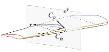
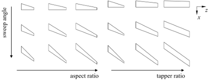
The single-segment swept wings are wings with the simplest planform geometries. A sketch diagram of the frontal, profile, and top views of a simple wing is depicted below.
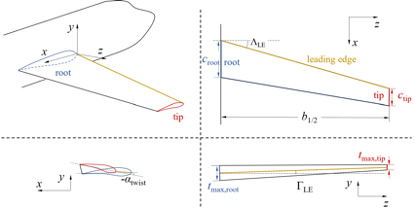
Its geometry is generated by linearly extruding the wing surface between the two control sectional airfoils on the tip and root.
Five planform geometry parameters are used to describe the wing: the tapper ratio (\(TR\)), aspect ratio (\(AR\)), leading-edge sweep angle (\(\Lambda_\text{LE}\)), leading-edge dihedral angle (\(\Gamma_\text{LE}\)), and tip-to-root twist angle (\(\alpha_\text{twist}\)). The are defined as:
Geometries of the kink wings
In engineering applications, it is difficult for a single-segment wing to fulfill its aerodynamic and structural / installation needs under multiple operating conditions, so a wing with a “yehudi break” or “kink” is always adopted as the planform geometry. The figure below shows the top view of a kink wing
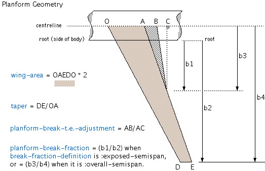
There are several extra parameters to control the kink part.
root adjustment: defined by \(\kappa = AB/AC\)
break location: defined by \(\eta_k = b_3/b_4\)
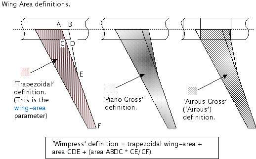
There are several ways to define the reference area (\(S_\text{ref}\)) of the kink wing as shown below. (from reference). Here we do not take the fuseluge into consideration, and the full wing area (denoted as “Piano Gross” in the figure) is used.
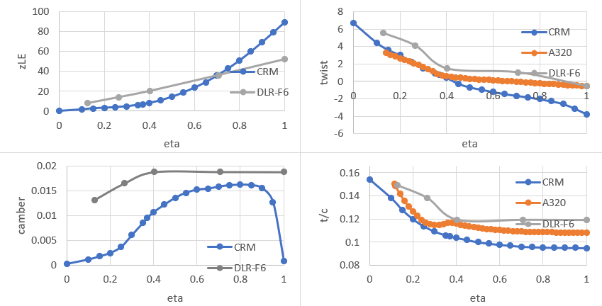
A brief summary of typical kink wing models
CRM |
DLR-F6 |
CHN-T1 |
Boeing 787 |
Airbus 320 |
|
|---|---|---|---|---|---|
cruise mach number |
0.85 |
0.75 |
0.85 / 0.9 |
0.775 |
|
nominal lift coefficient |
0.50 |
0.50 |
|||
Reynold number per ref. c. |
40 mil. |
37.6 mil. |
|||
aspect ratio |
8.38 (c) |
9.28 (c) |
9.20 |
8.79 (d) |
|
ref area |
0.1479 (c) |
374.257 |
120.7 (d) |
||
mean aero chord (tape) |
0.126 |
6.437 |
3.705 (d) |
||
taper ratio (tape) |
0.275 |
0.38 |
0.18 |
0.33 (d) |
|
1/4 chord sweep |
35 deg. |
25.15 deg. |
32.2 deg. |
25.0 deg. |
|
LE dihedral angle |
0.8 ~ 6.5 deg. (b) |
5.2 deg. |
6 deg. |
4.4 deg. (d) |
|
fuseluge location |
10% |
12.7% |
8% |
12% (d) |
|
kink location |
37% |
40.1% |
37.44% (a) |
39.2% (d) |
|
thickness kink location |
/ |
/ |
38.64% (a) |
38.11% (d) |
|
root adjustment |
67.2% |
100% |
88% |
100% (d) |
|
t/c center |
0.1542 |
0.1629 |
0.1449 (a) |
0.1394 (d) |
|
t/c break/center |
0.6822 |
0.7316 |
0.6472 (a) |
0.7166 (d) |
|
t/c tip/center |
0.6161 |
0.7306 |
0.6056 (a) |
||
inner twist (w.r.t center) |
-5.95 deg. (b) |
-4.11 deg. |
-3 deg. (b) |
-3 deg. (b,e) |
|
outer twist (w.r.t kink) |
-4.91 deg. (b) |
-2.03 deg. |
-3 deg. (b) |
-1.16 deg. (b,e) |
|
reference |
(d) (e) |
(a) originally defined with exposed ratio, transferred to overall ratio
(b) should be a distributed value
(c) originally wimpress or Airbus, transfered to Piano
(d) measured from figure
(e) measured from literature
Simple kink wings
B-1. Wings / Kink wings with DPW-W1 profile
This dataset contains two parts, the single-sigment simple wings and two-sigment “kink” wings. This dataset is mainly to study the influence wing planform parameters on model training, so the sectional airfoil of wings are fixed to be the Wing I in the AIAA Darg Prediction Workshop III (DPW3). The maximum relative thickness and tail relative thickness are 0.135 and 0.0004, respectively. There are 846 simple wings and 164 kink wings.
Their operating conditions (incl. Angle of Attack and freestream Mach number) also vary.
The dataset has been used in:
Citation:
Yang, Yunjia, Runze Li, Yufei Zhang, Lu Lu, and Haixin Chen. 2024. “Transferable Machine Learning Model for the Aerodynamic Prediction of Swept Wings.” Physics of Fluids 36 (7): 076105. https://doi.org/10.1063/5.0213830.
Sampling
Acting as the source domain of the transfer learning framework, the planform parameters of the wings in the simple wing dataset are sampled over a wide range of possible values as shown in Table.
Parameter |
Symbol |
lower bound |
upper bound |
|---|---|---|---|
sweep angle |
\(\Lambda_\text{LE}\) |
0° |
35° |
dihedral angle |
\(\Gamma_\text{LE}\) |
0° |
3° |
aspect ratio |
\(AR\) |
6 |
10 |
tapper ratio |
\(TR\) |
0.2 |
1.0 |
twist angle |
\(\alpha_\text{twist}\) |
0° |
-6° |
The straight wing that is without sweep, dihedral, tapper, and twist is used for one side of the boundary, while the other side of the boundary is determined by experience according to the typical values such as the values of the DPW-W1.
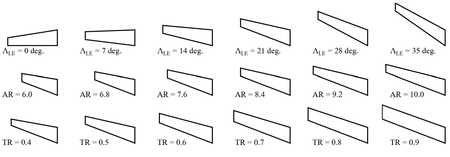
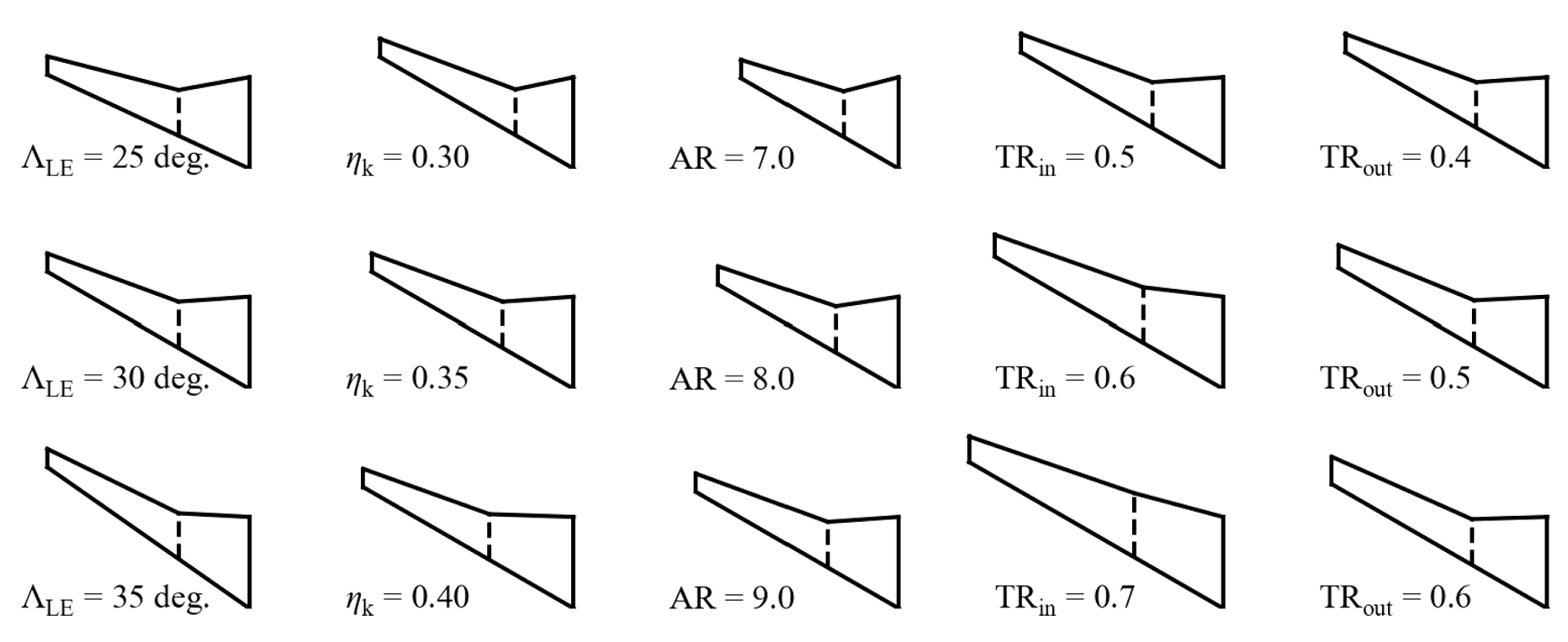
The kink wings are the target domain in the proposed transfer learning framework, so the ranges of the planform parameters in the dataset are decided based on typical values for commercial airliner’s wings.
Here, we focus on “simple” kink wings which can be seen as a concatenation of two simple wings that share the same leading-edge sweep and dihedral angle but have different tapper ratios and twist angles. Thus, we use another geometric definition here: The tapper ratios for the inner and outer segments are defined by \(c_\text{kink}/c_\text{root}\) and \(c_\text{tip}/c_\text{kink}\), and their twist angles are similarly defined by kink-to-root and tip-to-kink. \(\eta_k\) is introduced to describe the spanwise location of the kink.
Parameter |
Symbol |
lower bound |
upper bound |
|---|---|---|---|
sweep angle |
\(\Lambda_\text{LE}\) |
25° |
35° |
dihedral angle |
\(\Gamma_\text{LE}\) |
2° |
2° |
aspect ratio |
\(AR\) |
7 |
9 |
kink position |
\(\eta_k\) |
0.3 |
0.4 |
tapper ratio of the inner segment |
\(TR_\text{in}\) |
0.5 |
0.7 |
tapper ratio of the outer segment |
\(TR_\text{out}\) |
0.4 |
0.6 |
twist angle of the inner segment |
\(\alpha_\text{twist,in}\) |
-2° |
-4° |
twist angle of the outer segment |
\(\alpha_\text{twist,out}\) |
-2° |
-5° |
Grid
Grids were generated with CGrid.
Sectional airfoil grid:
Structured C-type grid solved with elliptic equation to ensure grid orthogonality
Grid size is 401×81 in the circumferential direction (i-direction) and wall-normal direction (j-direction).
The grid contains 321 cells on the airfoil surface. The far-field location is 80 chords away from the airfoil. The height of the first mesh layer is 2.7e-6 chord.

Wing grid:
Wing grid is obtained by linearly interpolate the sectional grid from tip to root
Spanwise grid has 61 points for simple wings; and 25 and 65 points for the inner and outer segments, respectively, for kink wings. The spanwise positions distributed more densely near the wing tip.
Grid points near the wing tip are extruded outside to form another grid block, as marked in red in figure.

the outermost layer of the grid is extruded to the far field (30 chords away) with 41 grid points.
Grid size: 2.86 million (single wings), 3.66 million (kink wings).
CFD
Computed using the Reynolds Average Navier–Stokes (RANS) solver CFL3D.
finite volume method
MUSCL scheme, ROE scheme
Gauss-Seidel algorithm
Turbulance model: shear stress transport (SST) model
Multigrid: three-level W-cycle multigrid: steps from coarse to fine 1000, 1000, and 6000
convergence criteria: lift coefficient in the last 500 steps is lower than 0.0002
final size: 846 for simple wings and 164 for kink wings
Data format
output surface flow field
file name |
|
|---|---|
array size |
Simple wing (846, 6, 321, 61) |
dim. 1 |
|
dim. 2 & 3 (flow field size) |
Simple wing 321 (around sectional airfoil) x 61 (spanwise**) |
* all geometry variables are DIMENSIONAL. Coefficents are on mesh points. Surface friction distributions are decomposed by in x-y plane and z-direction as follow:
** The values are linearly interpolated to a uniformly distributed series of z-position sections to unify the simple and kink wing data formats. The interpolated data can be found in wing101.npy
input wing parameters
There are two version index files: global parameters and distributed parameters. Global parameters are original planform parameter and operating conditions. Distributed parameters are local position, chord length, and AOA values at every cross-section that need to be predicted. We demonstrated in PoF 2024 distributed parameter inputs are better.
Global parameter file
file name |
Simple wing |
|---|---|
array size |
(846, 14) |
0 |
wing index |
1 |
aoa |
2 |
Mach number |
3 |
sweep angle |
4 |
dihedral angle |
5 |
aspect ratio |
6 |
tapper ratio |
7 |
twist angle |
8 |
tip-to-root thickness ratio (\(=1\)) |
9 |
reference area |
10 |
lift coeffcient * |
11 |
drag coeffcient * |
12 |
reconstructed lift coeffcient ** |
13 |
reconstructed drag coeffcient ** |
file name |
Kink wing |
|---|---|
array size |
(164, 17) |
0 |
wing index |
1 |
aoa |
2 |
Mach number |
3 |
sweep angle |
4 |
dihedral angle |
5 |
aspect ratio |
6 |
kink position |
7 |
tapper ratio of the inner segment |
8 |
tapper ratio of the outer segment |
9 |
tip-to-root thickness ratio (\(=1\)) |
10 |
twist angle of the inner segment |
11 |
twist angle of the outer segment |
12 |
reference area |
13 |
lift coeffcient * |
14 |
drag coeffcient * |
15 |
reconstructed lift coeffcient ** |
16 |
reconstructed drag coeffcient ** |
* read from clcd.dat from CFL3D calculation
** reconstructed from ground truth interpolated data (\(\approx 1\%\) error from CFD values) -> ground truth for coefficients in model training
Distributed input file
file name |
|
|---|---|
array size |
Simple wing (846, 101, 5) |
dim. 1 |
spanwise index |
dim. 2 |
|
xLE to zLE stands for position of the leading edge point of the sectional airfoil, chord represents the section chord, and alpha represents the effective alpha = wing alpha + twist angle.
B-2. Single Segment Wings
This dataset contains single-sigment simple wings with different airfoil profile, planform parameter, and operating conditions (incl. Angle of Attack and freestream Mach number). The wing’s cross-section profiles have the same CST parameters along spanwise, but the thickness is changed linearly. A total of 1842 wings are available now.
The dataset has been used in:
Citation:
Yang, Yunjia, Runze Li, Yufei Zhang, Lu Lu, and Haixin Chen. 2024. "Rapid aerodynamic prediction of swept wings via physics-embedded transfer learning". AIAA J, 2024
Sampling
sectional airfoil profile
The sectional airfoil are from dataset A-3, which contains 1420 airfoils with various performance. The maximum thickness of these airfoils are 0.08 ~ 0.14. Their thickness are transfered with swept theory according to swept angle when generating wings.
wing geometry
Each airfoil is used to construct two wings, and the wing planform parameters are randomly sampled from the range below:
Parameter |
Symbol |
lower bound |
upper bound |
|---|---|---|---|
sweep angle |
\(\Lambda_\text{LE}\) |
0° |
35° |
dihedral angle |
\(\Gamma_\text{LE}\) |
0° |
3° |
aspect ratio |
\(AR\) |
6 |
10 |
tapper ratio |
\(TR\) |
0.2 |
1.0 |
twist angle |
\(\alpha_\text{twist}\) |
0° |
-6° |
tip-to-root thickness ratio |
\(r_t\) |
0.8 |
1.0 |
operating conditions
AOA from 1 deg. to 6 deg., Mach from 0.72 to 0.85, Reynold number is 6.43 million, freestream temperature is 580 R.
Grids and CFD
Same to B-1
Data formats
output surface flow field
file name |
|
|---|---|
array size |
(1842, 6, 321, 61) |
dim. 1 |
|
dim. 2 & 3 (flow field size) |
321 (around sectional airfoil) x 61 (spanwise**) |
* ** same as B-1
input
Global parameter file
file name |
|
|---|---|
array size |
(1842, 35) |
0 |
wing index |
1 |
aoa |
2 |
Mach number |
3 |
sweep angle |
4 |
dihedral angle |
5 |
aspect ratio |
6 |
tapper ratio |
7 |
twist angle |
8 |
tip-to-root thickness ratio |
9 |
reference area |
10 |
root relative thickness |
11-20 |
CST coeffcients for upper surface |
21-30 |
CST coeffcients for lower surface |
31 |
lift coeffcient * |
32 |
drag coeffcient * |
33 |
reconstructed lift coeffcient ** |
34 |
reconstructed drag coeffcient ** |
* ** same as B-1
Distributed input file (sectional parameters)
Compared to B-1, distributed version geometry adds sectional airfoil profile to each cross section.
file name |
|
|---|---|
array size |
Simple wing (1842, 101, 27) |
dim. 1 |
spanwise index |
dim. 2 |
|
xLE to zLE stands for position of the leading edge point of the sectional airfoil, chord and thick represents the section chord and relative thickness. alpha represents the effective alpha = wing alpha + twist angle. cstu and cstl has 10 dimensions each, represent the CST parameters for the airfoil curves (in these dataset is the same). We also add a channel of Ma whose value is Mach number values every where.
Distributed input file (mesh points)
Another distributed version is to directly use the mesh points here, which is the first three channel of wing101.npy.
Auxilary files (for 2D prediction)
Normalized wing sectional profiles
The 2D model needs normalized (chord length to be 1 and no twist angle) sectional profiles of the wing sections to predict 2D flow field. Here we constructed a file that contains normalized airfoils.
file name |
|
|---|---|
array size |
Simple wing (1842, 101, 3, 321) |
dim. 1 |
spanwise index |
dim. 2 |
|
dim. 3 |
index around airfoil |
Sectional lift distribution
The sectional lift coefficient of each cross-section is obtained with
where \(L\) is the lift integrated from sectional pressure and friction distribution.
The sectional drag coefficient distribution can be defined similarly.
file name |
|
|---|---|
array size |
Simple wing (1842, 3, 101) |
dim. 1 |
|
dim. 2 |
spanwise index |
The original mesh grid version (with 61 spanwise points) can be found in wingcldistribution.npy
B-3. Kink Wings
This dataset contains kink wings with different airfoil profile, planform parameter (with curved thickness, camber, dihedral, and twist spanwise distribution), and operating conditions (incl. Angle of Attack and freestream Mach number). A total of ## wings are available now.
The dataset has been used in:
Citation:
##
Sampling
sectional airfoil profile
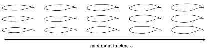
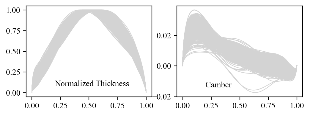
The CST coefficients of sectional airfoil are from dataset A-3, which contains 1420 airfoils with various performance. CST coefficients determine the thickness and camber distribution along streamwise. When using these CSTs to generate wings, at each spanwise location a maximum thickness and maximum camber is prescribed by spanwise thickness / camber distribution.
The normalized thickness and camber line are below:
wing geometry
Each airfoil is used as the reference sectional airfoil to construct two wings.
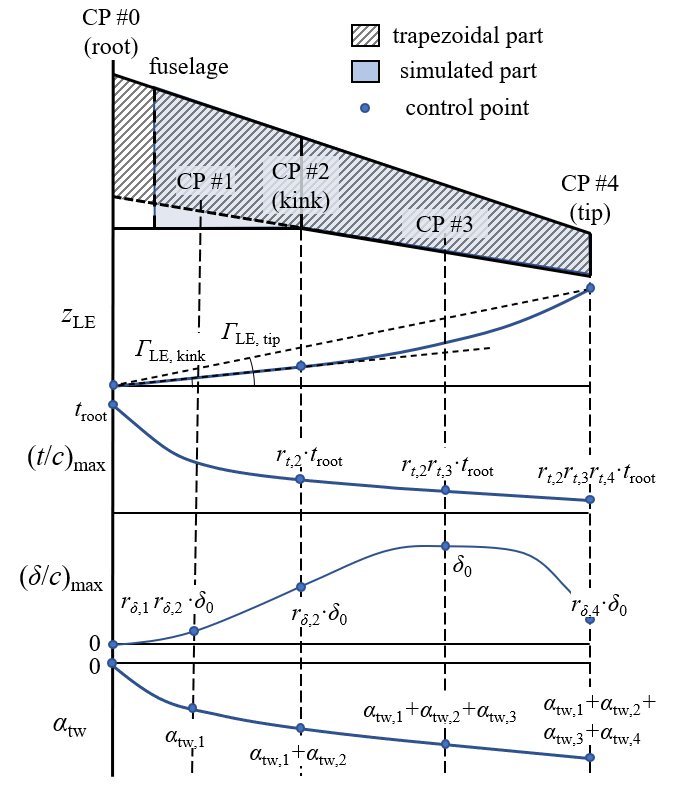
The projection shape of the wing is by first construct the trapezoidal part (marked by right slash lines) of the wing and then determin the kink and extra surface between root and kink.
The trapezoidal part is determined with the sweep angle, aspect ratio, and tapper ratio.
The extra surface is determined with the root adjustment ratio and kink location.
The fuselage line is fixed at 10%, and only the outer part of the wing (marked by light blue) are simulated.
The dihedral of the wing (on y axis) is distributed, and controled by two points at the kink and tip. It is linear between root and kink with the angle \(\tan(\Gamma_\text{LE,kink}) = y_\text{LE,kink}/z_\text{kink}\), the \(y_\text{LE, tip}\) at tip is decided with \(\Gamma_\text{LE,tip}\), and a Cubic Spline is constructed with kink, tip point and the slope at kink.
The sectional airfoil, as mentioned above, has the same CSTs spanwise, and spanwise-distributed max. thickness (\(t\)) and max. camber (\(\delta\)) are decided by Cubic Spline the link the control points (CPs).
The thickness has 4 CPs spanwise, locates at the root, kink, midpoint of kink and tip, and tip. The max. thickness values at these 4 CPs are \(t_\text{root}\), \(r_{t,2}\cdot t_\text{root}\), \(r_{t,2}r_{t,3}\cdot t_\text{root}\), \(r_{t,2}r_{t,3}r_{t,4}\cdot t_\text{root}\).
The camber has 5 CPs, with the extra one locates at the midpoint of root and kink. The sectional airfoil at the CP #3 has the same camber line of the reference airfoil. The camber line of the airfoil at CP #0, #1, #2, and #4 are linearly scaled with factors \(r_{\delta,1}r_{\delta,2}\), \(r_{\delta,2}\), and \(r_{\delta,4}\).
The twist angle of the wing also decided by 5 CPs. With CP #0 being zero, the twist angle at outer CPs are accumulated.
The wing planform parameters are randomly sampled from the range below:
Parameter |
Symbol |
lower bound |
upper bound |
|---|---|---|---|
sweep angle |
\(\Lambda_\text{LE}\) |
25° |
40° |
dihedral angle (tip) |
\(\Gamma_\text{LE, tip}\) |
4° |
6° |
dihedral angle (kink) |
\(\Gamma_\text{LE, kink}\) |
0.5° |
6° |
aspect ratio (trape.) |
\(AR\) |
8 |
11 |
tapper ratio (trape.) |
\(TR\) |
0.15 |
0.40 |
kink location |
\(\eta_\text{k}\) |
36% |
42% |
root adjustment |
\(\kappa_\text{root}\) |
50% |
110% |
root rela. thickness |
\(t_\text{root}\) |
0.14 |
0.17 |
spanwise thick. CP2 |
\(r_\text{t,2}\) |
0.60 |
0.70 |
spanwise thick. CP3 |
\(r_\text{t,3}\) |
0.90 |
0.98 |
spanwise thick. CP4 |
\(r_\text{t,4}\) |
0.92 |
1.00 |
spanwise camber CP1 |
\(r_{\delta,1}\) |
0.3 |
0.8 |
spanwise camber CP2 |
\(r_{\delta,2}\) |
0.5 |
1.0 |
spanwise camber CP4 |
\(r_{\delta,4}\) |
0.0 |
0.8 |
twist CP1 |
\(\alpha_\text{twist,1}\) |
-4° |
-2° |
twist CP2 |
\(\alpha_\text{twist,2}\) |
-4° |
-2° |
twist CP3 |
\(\alpha_\text{twist,3}\) |
-3° |
-1° |
twist CP4 |
\(\alpha_\text{twist,4}\) |
-3° |
-1° |